Robotic Motion Planning and Optimal Control

MPC hover recovery in simulation

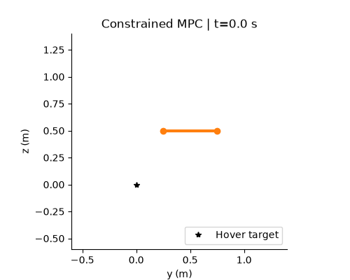
Planar quadrotor recovering from an offset position and velocity to a fixed hover target at the origin under MPC N=10. — One input-constrained MPC controller (N=10), over 10 simulated seconds. The blue curve is the traveled path toward a fixed hover target. Motor thrust is limited to 0–5.5 N per motor.

Reduced-motion preferences are respected. Pausing shows the starting frame; play to view the original animation.

Two controllers, the same nonlinear plant

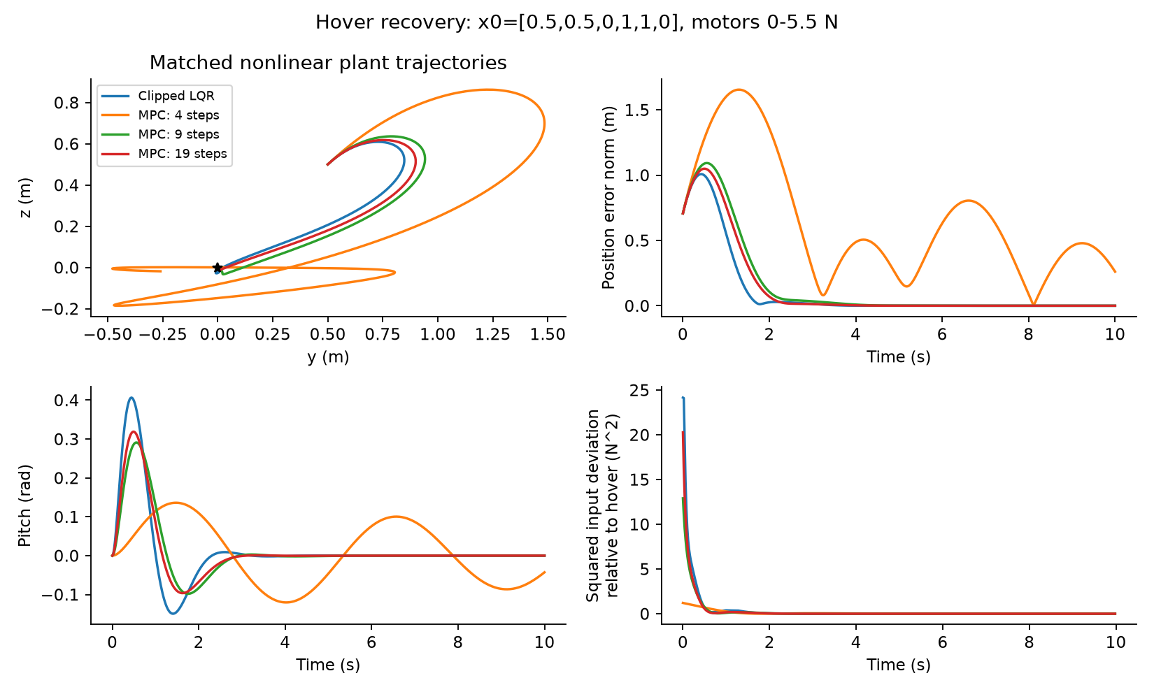
Input-constrained linear MPC plans a finite sequence of motor commands with a hover-linearized model and explicit thrust bounds. It applies the first command and replans at the next control update. Clipped LQR uses a continuous-time linear-quadratic feedback gain, then clips its commands to the same motor limits.

Both controllers run on the same nonlinear planar quadrotor, with identical initial conditions, integration, actuator limits and evaluation duration. The comparison examines the behavior of these specified configurations.

Four panels compare clipped LQR and MPC with 4, 9 and 19 predicted input steps: planar paths, position error, pitch angle and squared input deviation relative to hover. — Matched 10-second hover recovery. Short-horizon MPC does not settle in this example. Open the figure for full-size labels.

Results for initial state [0.5, 0.5, 0, 1, 1, 0]
Controller	Position RMSE (m)	Full-state settling (s)	Control effort relative to hover (N² s)
Clipped LQR	0.2873	2.68	3.8730
MPC N=5	0.7994	Not settled	0.8692
MPC N=10	0.3501	3.26	2.4021
MPC N=20	0.3257	2.62	2.8863

MPC N=10 uses 38.0% less control effort relative to hover, with 21.9% higher position RMSE and slower settling than clipped LQR in this configuration.

Control effort is the time integral of squared applied thrust deviation from nominal hover: ∫ ‖u(t) − u_hover‖² dt, with u_hover = [4.905, 4.905] N. It counts deviations in either direction and does not measure physical energy consumption.

LQR and MPC use different objective and terminal-cost conventions. The settings below make this a matched-plant comparison, not an isolated test of constraint handling.

Controller settings

Plant and rollout: state [y, z, θ, v_y, v_z, ω], initial state [0.5, 0.5, 0, 1, 1, 0]; mass 1 kg; moment arm 0.25 m; inertia 0.0625 kg m²; gravity 9.81 m/s². Nonlinear RK4 integration at 0.005 s; held control updates every 0.02 s; 10 s total; no disturbance in this displayed trial. The planar model omits ground collision and aerodynamic drag.
LQR: continuous infinite-horizon design with Q = diag(10, 10, 1, 1, 1, 1), R = I₂. No finite terminal cost; the CARE solution supplies the feedback gain. Applied commands are clipped to [0, 5.5] N per motor.
MPC: the same numerical Q and R in an unscaled discrete stage sum, terminal Q, forward-Euler prediction at 0.1 s. N counts states; N=10 has nine input steps and a 0.9 s prediction horizon. Motor bounds are imposed relative to hover.
Cost convention: multiplying the entire MPC objective by 0.1 leaves its optimizer unchanged and gives a rectangle-rule interpretation with terminal matrix 0.1Q, not Q or the CARE value matrix. These are not equivalent objectives.
Settling: all six absolute state errors must stay within [0.02, 0.02, 0.02, 0.05, 0.05, 0.05] in their respective SI units through the end of the finite run. Position RMSE is √mean(y² + z²), including the initial sample.
Verification: metrics were independently recomputed from saved applied-input traces. The unrounded comparison is 37.977996% lower effort and 21.869478% higher position RMSE.

Minimum-snap waypoint planning

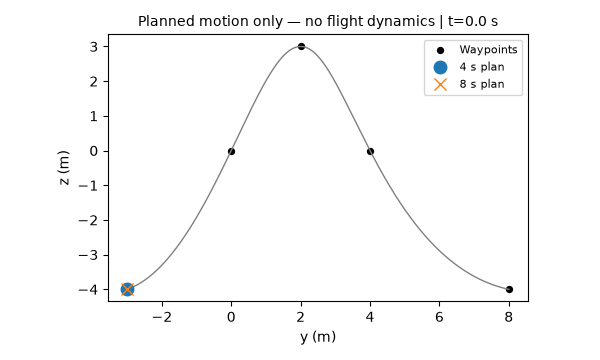
Plan piecewise-polynomial paths through five planar waypoints while minimizing the integral of squared snap—the squared fourth derivative of position. The solver enforces waypoint interpolation and continuity through the fourth derivative, with free endpoint derivatives.

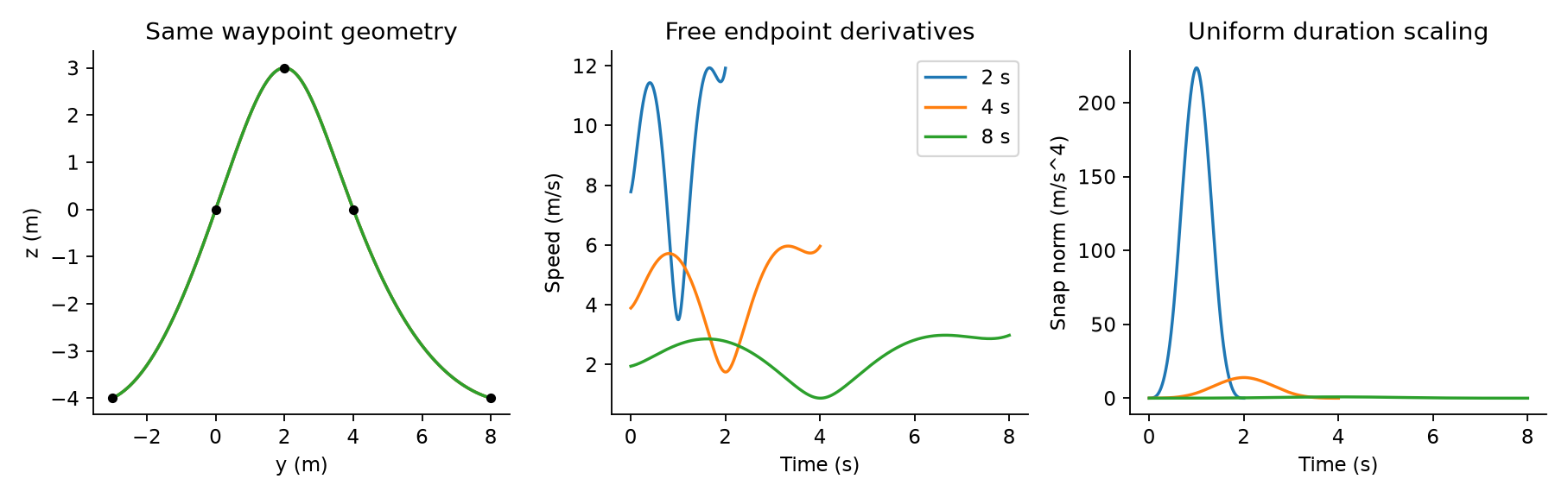
Minimum-snap paths for total durations of 2, 4 and 8 seconds overlap geometrically, while longer durations reduce speed and snap. — The same waypoint geometry at three durations. Endpoint velocity, acceleration and jerk are not fixed to zero.

Doubling total duration from 4 to 8 seconds reduces integrated squared snap by 128×, from 210.6954 to 1.6461. The geometric path is preserved; the objective scales as T⁻⁷. Independent numerical integration confirms the objective.

Formulation and numerical checks

Four degree-13 polynomial segments use 14 coefficients per coordinate in normalized local time. Waypoints are (−3, −4), (0, 0), (2, 3), (4, 0), (8, −4). Segment durations are uniformly 0.5, 1 or 2 s.

Row-scaled equality constraints and a nullspace least-squares solve avoid explicitly forming a squared-condition-number monomial Hessian. Per coordinate, the equality matrix has rank 20 over 56 coefficients. The snap operator has a 16-dimensional piecewise-cubic kernel; restricting the constraints to that kernel rules out a feasible zero-snap path for these waypoint timings. No endpoint conditions were added to force a nonzero objective.

Independent adaptive integration gives 210.6953642383607 for the 4 s path. Maximum waypoint residual is 1.12 × 10⁻¹⁴ m; the largest derivative-continuity residual is 6.91 × 10⁻¹¹ in its corresponding derivative units. Peaks in the figure are sampled, not certified continuous extrema. The geometric optimization uses free endpoint derivatives; thrust, tilt and obstacle constraints are outside its formulation.

Additional saved demonstrations

Cart-pole: energy shaping to LQR

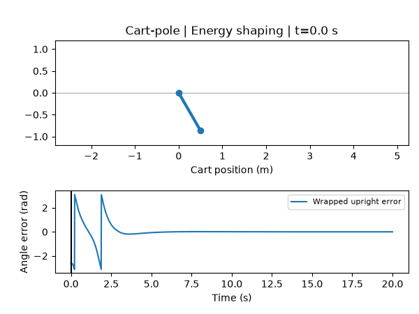
This 20 s nonlinear simulation starts 30° from downward rest. Energy shaping raises the pole, then switches once to local LQR at 2.79 s. The saved trajectory settles at 9.84 s: cart position and wrapped upright angle stay within 0.05 m and 0.05 rad, and both speeds within 0.1 in SI units, through the remaining run. The cart reaches 4.06 m from the origin, exceeding the ±2 m reference bound during the transient; cart travel is unconstrained in this simulation.

Cart-pole swing-up with energy shaping, followed by upright LQR stabilization; lower panel shows wrapped upright angle error. — Saved nonlinear cart-pole trajectory. Downward-zero pole angle; 1 m pole. The full transient and settling interval are shown at original simulation speed.

Minimum-snap: same geometry, different timing

Two planned point motions traverse the same waypoints in 4 and 8 seconds; the faster marker waits at the endpoint after 4 seconds. — Planned waypoint motion on one physical clock; the 4 s plan waits after completion. The geometric planner minimizes squared snap with free endpoint derivatives.

Optional modules: unicycle and iLQR

Secondary examples include unicycle flatness-based planning and quadrotor-pendulum iLQR. Their saved studies, solver status and endpoint checks are documented in the linked technical report.

Implementation contributions

Solver implementations: a portable sparse constrained-MPC QP and a scaled minimum-snap solver for the course formulations.
Model and simulation corrections: fixed the quadrotor integrator’s frozen-state callback; added held-input nonlinear simulation, full-state success checks and commanded/applied-input logging.
Numerical checks: verified hover and linearization, input-bound offsets, QP residuals, polynomial continuity, objective nullspaces and independent integration.
Reproducible experiments: recorded configurations, seeds, solver settings and numerical outputs for horizon, cost-weight, disturbance, mass-mismatch and duration studies.

Developed from Penn MEAM 5170, Fall 2025 coursework. The implementation adds a constrained-MPC solver, scaled minimum-snap solver, nonlinear simulation corrections, numerical checks and reproducible experiments using the supplied course models and frameworks.